Calculated Items in Pivot Tables

Work with Excel pivot tables long enough and you will find yourself suffering many frustrations. For starters, there’s no way to create your own AutoFormats, so unless your company wants to use Microsoft’s idea of good-looking tables as its standard format, you’re prett much stuck with copy/pasting and doing your own formatting. This is as of Excel 2003, of course.

But one of my biggest pet peeves, and one that I’ve actually been able – to some extent – to overcome, is the idea of creating my own formulas that will pivot and calculate the way any other data element in the report would. That’s a little vague, so I’ll give an example.

Right now my department is working on yearly assesments of the market shifts and demographics for 2007 (yes, it’s half-way through 2008, but that’s how long it takes to get the needed data from the state). There are a few calculations that have to be done on this data, including, but not limited to:

1. Since the data is still only current through the third quarter of 2007, the year of 2007 needs to be multiplied by 4/3 to annualize it for proper trending.
2. Each campus has its own overview, and groups competing hospitals differently. For my books, I need to look at our main campus, all of our campuses as a group, the three main competing hospitals as one group, and all the competition as one group.
3. For many of the campuses, we are looking at the tri-county and seven-county regions surrounding our hospital as a grouping for high-level analyses. The smaller campuses define primary and secondary service areas by zip codes (far more annoying).

All of these caluculations and groupings can be done using “Calculated Fields” and “Calculated Items”. Seems simple enough, but this feature hid itself from me for a long time.

Ok, so lets say you have a pivot table, created from a very simple data set of foodstuffs (carrots, milk, oranges, peas, tofu, and yogurt), some states where people eat these foodstuffs, and the number of people from each state who eat each foodstuff. It might look like this:

Sample Pivot Table

Now, say you want to group these states differently. You want to see FL, GA, AL, and LA grouped as the southeastern states. If your dataset is small enough and is already housed in excel, you can just overwrite the values of the states FL, GA, AL, and LA as “Southeast”, or create another column titled “Region” and fill in “Southeast” wherever applicable. But if you’re using a pivot table with over 65k records, this isn’t an option (Excel 2007 features an unrestricted number of rows, which will make a lot of this obsolete).

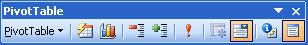
PivotTable Toolbar

Ever seen this window before? It’s the pivot table toolbar. It’s shown here as a modal window, but it can also be embedded into the main toolbar, of course, which is where I usually have it. If you don’t have this showing, just right-click on your pivot table and select “Show PivotTable Toolbar”.

Even if you have used this toolbar before, you might not have noticed that “PivotTable” drop-down on the left. There are some interesting things in there, like this:

You may have to click on appropriate fields in your pivot table first in order to access both Calculated Fields and Calculated Items. In my case, I clicked on one of the states first. Once you select Calculated Item, you get the following dialog box:

This shows the fields in my pivot table on the left, and the values available for the selected field on the right. This is not the same dialog box you get for a calculated item, because calculated fields assume you are using the values of a field to create a calculation, whereas calculated items use the items themselves. It’s a very fine line between the two, and I urge you to examine for yourself the subtle differences.

Anyway, on with the show. This is how I would create a grouping of the southeastern states:

Essentially, the field “Southeast” will contain the added values of whatever would have shown for AL, FL, GA, and LA. This remains true no matter how the table is pivotted (another distinction between this and calculated items). Once this is created, it shows as a regular item under the “State” field, as such:

Updated PivotTable

Now I am free to pivot as I see fit, and the “Southeast” value will always act as the simple sum of those four states, whether nested or not.

You may have noticed that adding a calculated item causes the totals to be “double-dipped”. This is yet another annoyance of pivot tables, but, really, how else would it be done? You are creating basically another item, and it needs to be included in the “Grand Total”. In our situation, we don’t need to see the southeastern states twice, we only need to see their grouped value. Simple enough, all we need to do is filter out the individual states by clicking the “State” drop-down and unchecking them, as such:

Now your pivot table will only show the non-southeast states and the Southeast grouping, ensuring that your totals will be correct, and all will be right with the universe.